Timsort - The Default Sort
Introduction
Timsort is used in the default .sort() implementations of at least 5 different languages. It exploits a crucial property of real-life data: it is often locally sorted in small stretches.
Algorithms like Quicksort and Mergesort just ignore this completely, assuming a completely random distribution. More formally, Timsort is able to capitalize on the low entropy of input arrays.
What are “runs”?
A “run” is a sequence that is either increasing or decreasing. For example in the array [8, 4, 2, 6, 11], [8, 4, 2] is a decreasing run of length 3.
Step 1 - Finding Runs
The first part of Timsort basically does this - scan from left to right for natural runs (either increasing or decreasing). For the array [8, 4, 2, 6, 11] that would be [[8, 4, 2], [6, 11]].
In practice, runs have a minimum length called min_run_length which the run is extended to.
For the example [8, 4, 2, 6, 11], if the min_run_length is 4, the first run [8, 4, 2] is shorter than min_run_length = 4, so it is extended by tacking 6 to the end of it - so the actual split into runs would look like [[8, 4, 2, 6], [11]].
All descending runs are then reversed. Since an extended array is almost sorted, insertion sort[1] is very efficient to turn this extended array into the sorted [2, 4, 6, 8].
In practice min_run_length = 32 or 64.
Animation of Step 1
Check out the animation below for running step 1 on the array [1, 3, 5, 7, 9, 8, 4, 2, 6, 11, 15, 13, 14] with min_run_length = 4.
We end up with 3 runs: [1, 3, 5, 7, 9], [2, 4, 6, 8], and [11, 13, 14, 15].
Pseudocode
The pseudocode for step 1 looks something like this:
runs = []
for each position in array:
    scan forward while asc/desc
    if the run was desc, reverse it in place

    if run length < min_run_length:
        extend the array
        perform insertion sort

    add run to runs
Step 2 - Merging the Runs
For those of you familiar with Mergesort - the next step should seem natural. It is quite simple to merge 2 sorted arrays, just start scanning from the left of the lists and take the smaller number. So all we need to do is repeatedly call merge on the runs to get bigger and bigger runs, until there is only 1 left.
Seems simple right? Well there is a small catch - the order of merging actually matters!
Why the Order Matters
Think of how many operations it takes to merge 2 sorted arrays of length m and n. It’s easy to convince yourself that this will take m + n operations in the worst case.
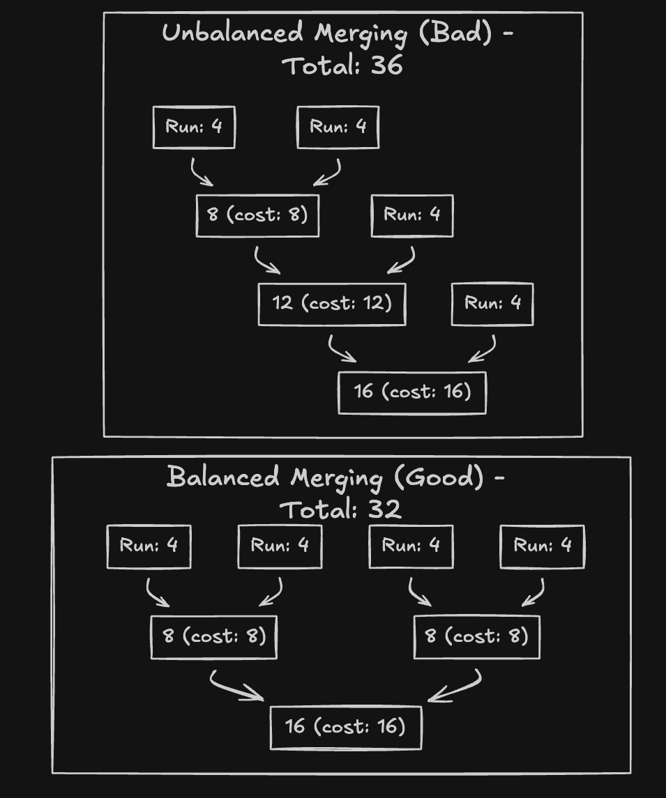
Since the cost is proportional to the length of the arrays, it makes sense to try and delay merging large arrays as much as possible. Below is an example of merging 4 runs of length 4.
The optimized merging tries to merge similar length arrays and delay large merges as much as possible, whereas the unoptimized approach naively merges.
The Stack Heuristic
Timsort uses a clever heuristic to merge equal length arrays and delay merging larger arrays.
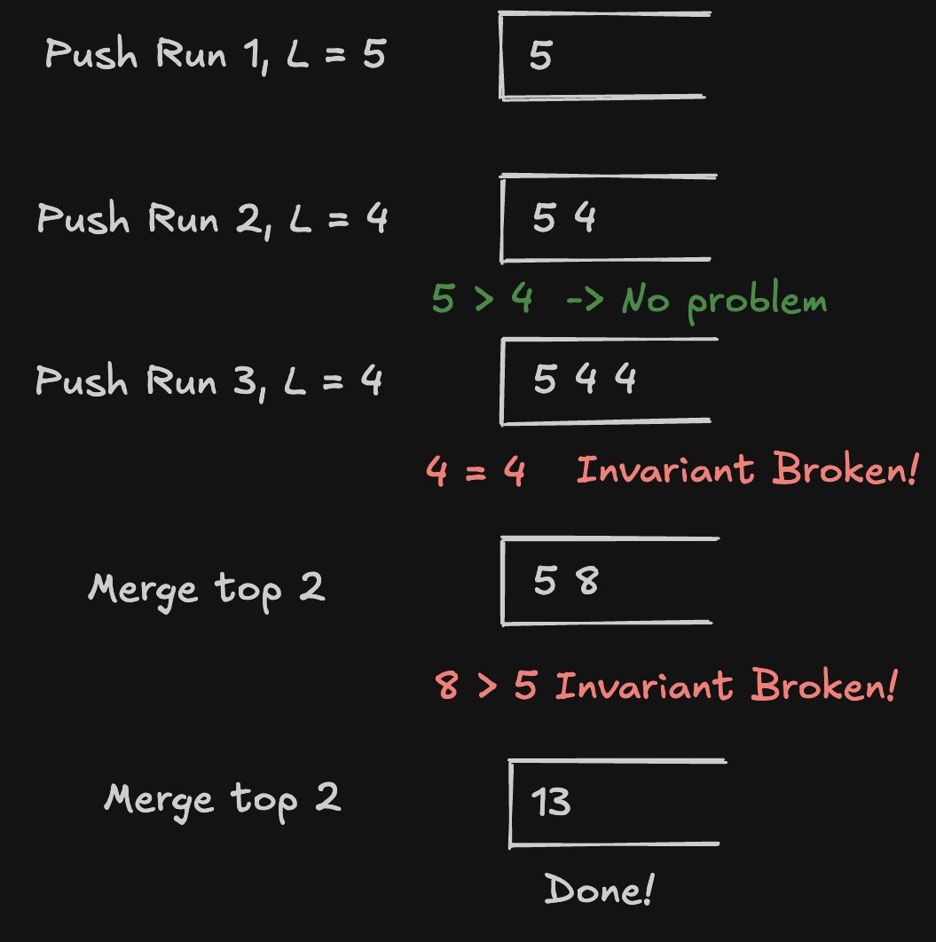
It uses a simple stack of runs. It tries to maintain the following invariants while pushing to the stack.
If stack[top - 2] = A, stack[top - 1] = B, stack[top] = C, then:
|A| > |B| + |C|- If this is violated, mergeBandC|B| > |C|- If this is violated, mergeAandB
This will naturally result in a decreasing stack, so larger arrays get merged last.
This ensures balanced merges similar to a balanced binary tree.
Example
Time Complexity
| Case | Complexity |
|---|---|
| Best (already sorted) | O(n) |
| Average | O(n log n) |
| Worst | O(n log n)[2] |
If the array is already sorted, it’s just a single run - terminating in O(n).
Meanwhile, Quicksort struggles with an already sorted array, taking its worst case O(n^2).
Mergesort does not exploit the sorted nature, making it take O(n log n) regardless.
Of course in the average/worst case, Timsort ends up taking O(n log n).
Footnotes
[1] The insertion sort mentioned above is actually binary insertion sort, which is an optimized O(n log n) version of insertion sort. ↩
[2] The stack heuristic is actually not optimal. There is a rare worst case that can be constructed to make Timsort take O(n^2). ↩